What is Interpolation Technique?
Interpolation is a technique used to estimate values within a range of data points. It is a common method used in many fields such as mathematics, computer science, physics, engineering, and many others. This blog will explore the concept of interpolation and its applications.
Interpolation involves estimating the value of a function at a point within the range of given data points. This can be done using different methods, such as linear interpolation, polynomial interpolation, spline interpolation, and many others.
Linear Interpolation
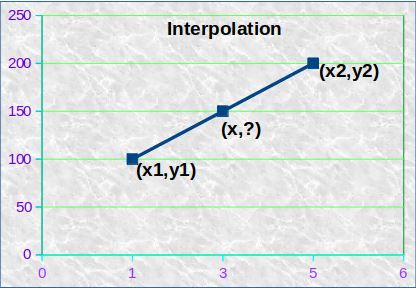
Linear interpolation is the simplest form of interpolation. It involves estimating the value of a function at a point using a straight line between two neighboring data points. For example, if we have two data points (x1, y1) and (x2, y2), we can estimate the value of the function at a point x within the range [x1, x2] as:
y = y1 + (x – x1) * (y2 – y1) / (x2 – x1)
This formula is based on the equation of a straight line (y = mx + b), where m is the slope of the line and b is the y-intercept. In this case, the slope is (y2 – y1) / (x2 – x1) and the y-intercept is y1.
Polynomial Interpolation
Polynomial interpolation involves estimating the value of a function at a point using a polynomial of degree n that passes through n+1 data points. This method is more accurate than linear interpolation but can be more computationally intensive. The polynomial can be represented as:
f(x) = a0 + a1 * x + a2 * x^2 + … + an * x^n
where a0, a1, a2, …, an are the coefficients of the polynomial. These coefficients can be found by solving a system of equations based on the given data points.
Interpolation
Spline interpolation is a more advanced method that involves estimating the value of a function at a point using piecewise polynomial functions that are continuous and have continuous derivatives up to a certain order. This method is particularly useful when the data points have large variations and cannot be accurately represented by a single polynomial function.
Interpolation has many applications in various fields. In mathematics, interpolation is used to estimate the value of a function at a point where the function is not defined. In computer graphics, interpolation is used to generate smooth curves and surfaces. In engineering, interpolation is used to estimate the behavior of materials or structures under different conditions.
Linear Interpolation Example
Let’s say we have the following data points:
(x1, y1) = (2, 5) (x2, y2) = (6, 11)
We want to estimate the value of the function at x = 4 using linear interpolation.
Using the formula for linear interpolation, we can calculate the value of y as:
y = y1 + (x – x1) * (y2 – y1) / (x2 – x1)
Substituting the values we have:
y = 5 + (4 – 2) * (11 – 5) / (6 – 2)
Simplifying the expression:
y = 5 + 2 * 6 / 4
y = 8
Therefore, the estimated value of the function at x = 4 is 8. This means that we assume the function behaves linearly between the two given points (2, 5) and (6, 11) and we can estimate the value at any point within this range.
Practical Example 1
One practical example of linear interpolation is estimating the temperature at a specific time based on two temperature measurements taken at different times.
Let’s say we have the following temperature measurements:
| Time (hours) | Temperature (°C) |
|---|---|
| 0:00 | 15° |
| 6:00 | 22° |
| 12:00 | 29° |
We want to estimate the temperature at 9 am, which is 9 hours after the initial measurement was taken.
Using linear interpolation, we can estimate the temperature at 9 am by calculating the value of temperature between the two data points that surround this time. The two data points we will use for linear interpolation are:
(x1, y1) = (6, 22) (x2, y2) = (12, 29)
Using the formula for linear interpolation, we can calculate the temperature at 9 am as:
Temperature at 9 am = y1 + (x – x1) * (y2 – y1) / (x2 – x1)
Substituting the values we have:
Temperature at 9 am = 22 + (9 – 6) * (29 – 22) / (12 – 6)
Simplifying the expression:
Temperature at 9 am = 22 + 3 * 7 / 6
Temperature at 9 am = 25.5 °C
Therefore, the estimated temperature at 9 am is 25.5 °C, based on the linear interpolation of the temperature measurements taken at 6 am and 12 pm.
Practical Example 2
Let’s say you have a data set that represents the number of website visitors per day for a particular website over a period of time. You want to estimate the number of visitors for a specific date that falls in between two dates for which you have actual visitor data.
For example, let’s say you have the following data:
| Date | Visitors |
|---|---|
| 1 | 100 |
| 5 | 200 |
| 9 | 300 |
You want to estimate the number of visitors for the date 3.
Using linear interpolation, you can estimate the number of visitors for date 3 by calculating the value of visitors between the two data points that surround this date. The two data points we will use for linear interpolation are:
(x1, y1) = (1, 100) (x2, y2) = (5, 200)
Using the formula for linear interpolation, we can calculate the number of visitors for date 3 as:
Visitors for date 3 = y1 + (x – x1) * (y2 – y1) / (x2 – x1)
Substituting the values we have:
Visitors for date 3 = 100 + (3 – 1) * (200 – 100) / (5 – 1)
Simplifying the expression:
Visitors for date 3 = 100 + 2 * 100 / 4
Visitors for date 3 = 150
Therefore, the estimated number of visitors for date 3 is 150, based on the linear interpolation of the visitor data for dates 1 and 5.
In conclusion, interpolation is a powerful technique that allows us to estimate values within a range of data points. Different methods of interpolation can be used depending on the nature of the data and the required accuracy. Interpolation has a wide range of applications in various fields, and its importance cannot be overstated. Below is a free Excel file with linear interpolation example.

